qsv viz gallery (An Interactive Viz is worth a Million Rows)

smart dashboard (--smarter, geospatial)One command, 13 auto-chosen panels — nearly every panel type at once on a synthetic catalog of Japanese earthquakes. Things the raw table hides but the dashboard makes obvious: depth_km is bimodal (two populations — shallow interplate quakes ~20 km and the deep Wadati-Benioff slab ~450 km — so --smarter draws a histogram, not a box that would average the peaks away); the points trace Japan's subduction arcs on the map; and a prefecture choropleth bins each quake into the GeoJSON region that contains it (point-in-polygon, no geocoding). Most of this catalog is offshore Pacific seismicity, so under the default 10 km snap cap the far-offshore quakes are dropped (287 of 417 here — the panel title reports it) and the on-land/near-coast prefectures are colored; raise --snap-max-dist to snap distant quakes to the nearest prefecture instead, or --no-snap to drop every offshore point. magnitude vs felt_reports is almost perfectly correlated (r=0.95); magnitude and felt_reports are right-skewed with flagged outliers; and the magnitude-over-time trend spikes during a September aftershock sequence. --bivariate adds an NMI association heatmap spanning every column type, not just the continuous-numeric ones the Pearson heatmap covers — it surfaces depth_km and felt_reports as strongly associated with occurrence_date (NMI=0.93 and 0.89), a temporal-clustering signal (the same September aftershock sequence) a Pearson matrix restricted to numeric pairs alone cannot express against a date column. Coordinate columns are shown on the map only, not re-charted as distributions. Rendered with the built-in plotly_dark theme.

qsv viz smart seismic_events.csv --smarter --bivariate --theme plotly_dark \
  --grid-cols 3 --geojson japan_prefectures.geojson -o smart_dashboard_smarter_geospatial.html

smart dashboard (geographic outliers)Delivery stops clustered in metro Denver with four bad-geocode strays. Points far from the cluster centroid (beyond the Tukey far-out fence of their distances) are flagged as geographic outliers: drawn as distinct amber markers, drawn outside the purple (filled) spatial-extent box, and excluded from the auto-zoom — so the default view stays tight on the core cluster. A second, dashed-magenta no-fill box marks the full extent (core + outliers); use the Core extent / Full extent buttons at the top-left of the map to jump between the tight core view and the full spread (where the strays and the magenta box become visible). In the full qsv viz smart HTML output the spatial-extent label calls them out — Colorado, United States — 4 outliers (Wyoming, Kansas & Nebraska) — while strays within the core's own jurisdiction are folded back in silently instead. Each stop also carries delivery attributes (packages, weight_kg, distance_km, delivery_minutes, a vehicle class and a delivered_date), so beyond the map the auto-profiler fills the dashboard out with box plots, frequency bars, a correlation heatmap, the strongest-pair scatter (packages vs weight_kg) and a delivered-over-time trend — all without --smarter.

qsv viz smart delivery_stops.csv -o smart_dashboard_geographic_outliers.html

smart dashboardAuto-profiled overview: correlation heatmap + box plots + frequency bars, led by a drill-down sunburst. `viz smart` now SKIPS an auto hierarchy when the candidate dimensions are statistically independent (nesting them would just replicate each level's marginal); sales_sample's region/payment_method/product_category are independent, so `--hierarchy-style sunburst` is passed to deliberately showcase the interactive sunburst.

qsv viz smart sales_sample.csv --hierarchy-style sunburst --max-charts 8 \
  -o smart_dashboard.html

smart dashboard (KPI gauges & target delta)The KPI overview row driven by a hand-authored `--dictionary` (sales_kpi_dict.schema.json). Two optional `x-qsv` hints turn plain measure tiles into richer KPIs: a `gauge_range` of [0,1] draws Discount % and Profit Margin % as GAUGES on their canonical ratio scale, and a `target` of 0.25 on Profit Margin adds a "vs target" DELTA (the mean is 0.21, so a red -0.042 below the goal). qsv keeps a gauge only when the data lies within its range, so a mis-scaled range can't mislead; `gauge_range` is what `--dictionary infer` emits for canonical-scale ratios, while `target` is a business goal you hand-author (never LLM-inferred). Overall dataset completeness rides quietly in the header table, not as a tile.

qsv viz smart sales_sample.csv --dictionary sales_kpi_dict.schema.json \
  -o smart_dashboard_kpi_gauges_target_delta.html

smart dashboard (--smarter)Same auto-profiler with `--smarter`, which runs `qsv moarstats --advanced` itself to enrich the stats cache in one step: the bimodal monthly_spend column renders as a histogram (a box plot would hide its two peaks), and the skewed account_age_days box is annotated with its skew direction and outlier share.

qsv viz smart customer_spend.csv --smarter --max-charts 8 -o smart_dashboard_smarter.html

smart dashboard (--smarter, Gini/Lorenz inequality + log-skew boxes)Medicare payments to individual practitioners (CMS — a 30k sample), with medical_payment and total_patients per provider. These are additive amounts across comparable units, so --smarter recognizes them as inequality measures and adds a Lorenz curve for each (Gini 0.65 / 0.61) — the further the curve bows below the diagonal, the more concentrated the payments. The distribution boxes are skew-aware: a heavily right-skewed money column would squash a linear box into a sliver against its largest values, so viz smart draws it on a log axis instead, keeping the median and quartiles legible.

qsv viz smart cms_medicare_providers.csv --smarter -o smart_dashboard_smarter_gini_lorenz_inequality_log_skew_boxes.html

barRevenue by region (aggregated sum).

qsv viz bar sales_sample.csv --x region --y revenue --agg sum \
  -o bar.html

bar (animated slider)Revenue by product category, animated over an ordinal column with --slider: each distinct satisfaction rating (1–5) becomes an animation frame, with a ▶ Play/⏸ Pause button and a scrub slider to step through them (Gapminder-style). Axis ranges are pinned across frames so the bars stay comparable frame to frame instead of rescaling. --slider also works on line and scatter, may be split into animated traces with --series, and can accumulate with --slider-cumulative.

qsv viz bar sales_sample.csv --x product_category --y revenue \
  --agg sum --slider satisfaction -o bar_animated_slider.html

lineClosing price over time.

qsv viz line stock_prices.csv --x date --y close -o line.html

scatterUnits sold vs revenue.

qsv viz scatter sales_sample.csv --x units_sold --y revenue -o scatter.html

scatter (bubble)Units vs revenue; marker size = shipping cost, color = profit margin %.

qsv viz scatter sales_sample.csv --x units_sold --y revenue --size shipping_cost \
  --color profit_margin_pct -o scatter_bubble.html

scatter3dUnits vs revenue vs shipping cost in 3D; marker color = profit margin %.

qsv viz scatter3d sales_sample.csv --x units_sold --y revenue \
  --z shipping_cost --color profit_margin_pct -o scatter3d.html

histogramDistribution of unit price.

qsv viz histogram sales_sample.csv --x unit_price -o histogram.html

boxSpread of revenue (Tukey whiskers; points beyond the fences shown as outliers).

qsv viz box sales_sample.csv --y revenue -o box.html

box (grouped)Revenue spread per region — real Tukey whiskers + every (jittered) point overlaid (--box-points all).

qsv viz box sales_sample.csv --y revenue --x region --box-points all \
  -o box_grouped.html

violinRevenue distribution per region — a KDE density silhouette around an inner quartile box + mean line, revealing shape (modes, shoulders) a box hides. viz smart auto-picks this for columns in the bimodality ambiguity band (--violin auto).

qsv viz violin sales_sample.csv --y revenue --x region -o violin.html

pie (donut)Revenue share by product category.

qsv viz pie sales_sample.csv --x product_category --y revenue \
  --donut -o pie_donut.html

heatmap (correlation)Pearson correlation matrix over numeric columns.

qsv viz heatmap sales_sample.csv -o heatmap_correlation.html

scatter (correlated pair)The most strongly correlated numeric pair (discount_pct vs profit_margin_pct, r=-0.99). viz smart auto-adds this as a drill-down beside the correlation heatmap.

qsv viz scatter sales_sample.csv --x discount_pct --y profit_margin_pct \
  -o scatter_correlated_pair.html

contour2D density of units sold vs revenue (binned into a 20x20 grid). viz smart uses this instead of the pair scatter for large datasets, where a scatter would overplot.

qsv viz contour sales_sample.csv --x units_sold --y revenue --bins 20 \
  -o contour.html

heatmap (pivot)Region x category grid of revenue.

qsv viz heatmap sales_sample.csv --x region --y product_category \
  --z revenue -o heatmap_pivot.html

candlestickOHLC price action.

qsv viz candlestick stock_prices.csv --x date --ohlc-open open \
  --high high --low low --close close -o candlestick.html

ohlcOpen-high-low-close bars.

qsv viz ohlc stock_prices.csv --x date --ohlc-open open --high high \
  --low low --close close -o ohlc.html

radarMulti-axis brand comparison (per-axis mean per series).

qsv viz radar product_ratings.csv --cols battery,camera,performance,display,value,design \
  --series brand -o radar.html

sankeyWeb session funnel (duplicate edges aggregated).

qsv viz sankey web_flows.csv --source source --target target \
  --value sessions -o sankey.html

treemapPart-to-whole spend by plan then region, sized by summed monthly_spend. Rounded tiles + white separators come from the treemap-specific marker; non-numeric/negative measure cells are rejected so proportions can't silently misstate.

qsv viz treemap customer_spend.csv --cols plan,region --value monthly_spend \
  --agg sum -o treemap.html

sunburstThree-level hierarchy (region -> product_category -> payment_method) as concentric rings, sized by row count; inner rings are parents, outer rings their children. Opens at two rings (maxdepth) so labels stay legible instead of crowding a ~100-sector outer ring; click a sector to drill in and the deeper ring's labels grow back. Hover always shows value + percent.

qsv viz sunburst sales_sample.csv --cols region,product_category,payment_method \
  -o sunburst.html

icicleSame three-level hierarchy (region -> product_category -> payment_method) as a rectangular icicle: parents on the left, children fanning right, each rectangle sized by row count. The flat left-to-right layout keeps deep labels readable where a sunburst's outer ring would crowd; click a rectangle to zoom into that branch. Hover shows label + value + percent of parent.

qsv viz icicle sales_sample.csv --cols region,product_category,payment_method \
  -o icicle.html

splomScatter-plot matrix of four numeric columns (units_sold, revenue, discount_pct, profit_margin_pct): every pairwise scatter in an N x N grid with shared axes, so correlation structure is legible at a glance. viz smart auto-adds this panel when 3+ correlated numeric columns exist, capped at 6 dims selected by correlation participation.

qsv viz splom sales_sample.csv --cols units_sold,revenue,discount_pct,profit_margin_pct \
  -o splom.html

parcatsParallel-categories flow over three categorical columns (region -> product_category -> payment_method): each ribbon is a category combination, sized by how many rows share it, so co-occurrence between the dimensions is visible without implying a part-to-whole nesting. Ribbons are colored by their first-axis category and bundled (like a Sankey), and each axis opens ordered by frequency with a ⇅ category order toggle that flips every axis between frequency and alphabetical order. viz smart auto-adds this panel for 3-4 associated many-to-many categoricals (and suppresses the hierarchy on the same columns); genuine rollup trees still auto-select a treemap/sunburst.

qsv viz parcats sales_sample.csv --cols region,product_category,payment_method \
  -o parcats.html

mapEarthquake points on token-free OpenStreetMap tiles; marker color = magnitude, size = depth.

qsv viz map quakes.csv --lat lat --lon lon --color magnitude \
  --size depth_km -o map.html

map (density)DensityMap heatmap of the same points on a light Carto basemap, weighted by magnitude (via --color) so stronger quakes glow hotter — hovering a point shows its magnitude, not just the coordinates.

qsv viz map quakes.csv --lat lat --lon lon --density --color magnitude \
  --style carto-positron -o map_density.html

geoSame earthquakes on an offline natural-earth projection (no tiles, no token); marker color = magnitude. viz smart auto-uses this projection for global-extent coordinates.

qsv viz geo quakes.csv --lat lat --lon lon --color magnitude \
  --projection natural-earth -o geo.html

geo (animated slider)An animated point map: --slider steps through the region column, revealing the world's seismicity continent by continent, each region in its own color via --series. With --slider-cumulative the points accumulate as the animation plays (Play/Pause + a scrub slider). Unlike the MapLibre tile map, scattergeo animates natively, so --slider is supported on viz geo — use it instead of viz map for animated point maps.

qsv viz geo quakes.csv --lat lat --lon lon --slider region --series region \
  --slider-cumulative --projection natural-earth -o geo_animated_slider.html

choroplethFilled-region map coloring countries by GDP, matched by ISO-3 code on a token-free projection basemap. Use --location-mode usa-states / country-names / geojson-id for other region keys, --map for a MapLibre tile basemap, or --geocode to derive codes from lat/lon or place names.

qsv viz choropleth country_stats.csv --locations iso3 --value gdp_usd_tn \
  --color-scale viridis -o choropleth.html

choropleth (US states)Same chart, --location-mode usa-states: state codes matched to Plotly's built-in US-state geometry on the token-free albers-usa projection (CONUS + Alaska/Hawaii insets) — no GeoJSON needed. States are colored by renewable-electricity share.

qsv viz choropleth us_state_stats.csv --locations state --value renewable_electricity_pct \
  --location-mode usa-states -o choropleth_us_states.html

choropleth (MapLibre + GeoJSON)--map draws the filled regions on an interactive MapLibre tile basemap (token-free carto-positron) instead of a projection. The regions come from a custom GeoJSON (--geojson local file or URL) matched to the data by --feature-id-key — here the near-rectangular western states, colored by installed wind capacity. The view auto-centers and zooms to the GeoJSON extent (shown full-width so the computed zoom frames the regions as the CLI does — a tile map's zoom is fixed, so a narrow grid cell would crop it).

qsv viz choropleth western_states.csv --locations state --value wind_capacity_gw \
  --geojson western_states.geojson --feature-id-key id --map --style carto-positron \
  -o choropleth_maplibre_geojson.html

smart dashboard (time-series)Auto dashboard for stock_prices: a time-series trend panel (the first numeric column over the date) leads; the strongest-correlated pair drill-down (open vs close) is shown as a static scatter — that relationship is a near-perfect line whose 2-D shape doesn't evolve, so the judicious animation gate withholds the (uninformative) animated version — alongside box-plot summaries of the OHLC columns.

qsv viz smart stock_prices.csv --max-charts 8 -o smart_dashboard_time_series.html

smart dashboard (per-US-state choropleth)`viz smart` reverse-geocodes each point; because every city resolves to a US state, it adds a per-US-state choropleth (cities-per-state, albers-usa) beside the point map, alongside the usual box plots, frequency bars and the strongest-pair scatter. (The point map's spatial extent caption counts the data's bounding-box corners, which spill into neighboring countries and ocean — the choropleth instead resolves each city to its own state.) No flags, no LLM — the state fill is derived purely from the lat/lon columns.

qsv viz smart us_cities.csv -o smart_dashboard_per_us_state_choropleth.html

smart dashboard (--dictionary infer, treemap)Auto dashboard for customer_spend with a describegpt-inferred Data Dictionary (--dictionary infer) guiding panel selection & field labels. Two categorical dimensions (plan, region) form a shallow part-to-whole hierarchy, auto-rendered as a TREEMAP (area = size). Requires a local LLM; the committed HTML is reused on regen.

qsv viz smart customer_spend.csv --dictionary infer -o smart_dashboard_dictionary_infer_treemap.html

smart dashboard (--dictionary infer, sunburst)Auto dashboard for sales_sample with a describegpt-inferred Data Dictionary. Its three categorical dimensions are statistically independent, so the auto-profiler skips the hierarchy by default; `--hierarchy-style sunburst` forces a SUNBURST here (concentric rings emphasize parent-child structure) to showcase the chart. Requires a local LLM; the committed HTML is reused on regen.

qsv viz smart sales_sample.csv --dictionary infer --hierarchy-style sunburst \
  -o smart_dashboard_dictionary_infer_sunburst.html

smart dashboard (--dictionary infer, world choropleth)1,179 cities with population over 500,000 across six inhabited continents (GeoNames-derived): `viz smart` reverse-geocodes every point and adds a per-country choropleth (cities-per-country, ISO-3) framed to the filled-country geometries via Plotly fitbounds — so the regions are never clipped at the viewport edge — beside the dense natural-earth point map (crimson markers so coastal/island points read against the ocean), plus a six-continent breakdown. A describegpt-inferred Data Dictionary supplies the friendly field labels (e.g. Metro Population, Avg Annual Temp). The continent column follows the plotly.js geo scope continent vocabulary (Oceania, North America, …). Note: elevation_m is real (GeoNames), while avg_annual_temp_c is a rough synthetic proxy (latitude + elevation-lapse model), so treat it as illustrative. Requires a local LLM; the committed HTML is reused on regen.

qsv viz smart world_cities.csv --dictionary infer -o smart_dashboard_dictionary_infer_world_choropleth.html

smart dashboard (--smarter, committed --dictionary, NYC 311 metro choropleth)A 10,000-row sample of NYC 311 service requests (2010–2020) profiled into auto-chosen panels on a real, wide municipal dataset. The headline panel is the metro choropleth: each request's lat/lon is binned into NYC's 188 neighborhood polygons (no geocoding — 110 of them receive requests, and 10 of the 7,464 located points fall too far from any polygon to snap), and because the matched regions span a city-scale extent, viz smart draws the filled regions on an interactive MapLibre tile basemap (token-free carto tiles, fine street/coastline detail) instead of the coarse projection basemap it uses for country/continental choropleths. The leading point map flags bad-geocode outliers (here, 9 in Pennsylvania): a nice illustration of the hover's value — for a stray PA point, the tooltip shows the record's own Incident City: NEW YORK right above its reverse-geocoded Pennsylvania, United States, so a real Manhattan complaint saddled with corrupt coordinates is self-evident at a glance. --smarter runs moarstats --advanced to enrich the stats cache, and a committed --dictionary (nyc311_dict.schema.json — a Data Dictionary generated for this dataset, then reviewed and committed alongside it) tags the record's identifier columns (Unique Key, BBL) so they're skipped rather than charted as quantities, labels the State-Plane coordinates as coordinate dimensions, and supplies friendly names (e.g. Complaint Creation Date, Resolution Deadline), so the profiler treats a service-request log as volume-and-category data. Alongside the maps the auto-profiler fills the dashboard with frequency bars, an hour-of-day seasonality profile, a time trend, a parallel-categories (parcats) flow over 3-4 associated categorical columns (co-occurrence ribbons, auto-chosen over a nested treemap/sunburst for this many-to-many set) and a mean-by-borough panel. New here is an auto-selected, colored Sankey flow (Agency Code → Submission Channel): it traces how each city agency's complaints arrive by channel, the thickest ribbons being HPD → PHONE (1,426) and NYPD → PHONE (1,348). --bivariate adds an NMI association heatmap across the 36 charted columns plus a ranked Top Relationships panel — a horizontal multivariate lollipop where each dot's position is the pair's NMI on a value axis zoomed to the shown band (so near-ceiling associations separate instead of crushing together at 1.0), its size encodes co-occurrence support, and an amber dot flags a nonlinear pair. The top pair is a purely categorical one a Pearson-only heatmap could never surface, since neither column is numeric: Borough × Park Borough (NMI=1.0, n=10,000 of 10,000). It also flags a genuine nonlinear pair in amber — Closed Date × Due Date (NMI=0.9994): a complaint's actual close date is almost perfectly rank-associated with its deadline, yet how far the two land apart varies by complaint type, curving the relationship in a way a linear correlation alone would understate. The ranking is support-weighted: a pair only qualifies when its co-occurring row count is at least 10% of the best-supported pair's, so a technically-perfect NMI from two sparsely-populated columns can't crowd out a more broadly meaningful one — the top of the ranking instead surfaces genuinely dataset-wide pairs like Borough × Park Borough (n=10,000) and Due Date × Resolution Action Updated Date (NMI=0.9996, n=3,467). --dict-info adds a per-panel info icon and a slide-over Data Dictionary drawer sourced from the same committed schema, with an Export JSONSchema download that saves the dictionary verbatim. The run stays fully deterministic and offline: because the dictionary is committed, --bivariate never triggers a live --dictionary infer pass.

qsv viz smart nyc_311.csv --smarter --bivariate --dict-info --dictionary nyc311_dict.schema.json \
  --geojson nyc_neighborhoods.geojson -o smart_dashboard_smarter_committed_dictionary_nyc_311_metro_choropleth.html

smart dashboard (--smarter, curated --dictionary, region-code zip choropleth)All 50,013 Allegheny County lifetime dog licenses, profiled into auto-chosen panels. The headline panel is a summary choropleth keyed off a region-code COLUMN, not coordinates: this dataset has no lat/lon, only an OwnerZip column, so viz smart aggregates licenses per zip and fills the matching Allegheny County zip-boundary polygons from --geojson (--feature-id-key properties.ZIP). The key column is auto-chosen by matching each geo-dimension column's values against the boundary ids — here 118 zips match, from 1 license (rural fringe) to 2,866 in zip 15237 (suburban North Hills). Because the matched regions span a metro-scale extent, the fill lands on an interactive MapLibre tile basemap (token-free carto tiles) rather than the coarse projection basemap used for country/continental choropleths. A curated --dictionary (allegheny_dogs_dict.schema.json) tags OwnerZip as geo.zip_code — the signal that turns a numeric zip code into a choropleth key instead of a frequency bar — and marks _id/DogName as identifiers so they're skipped. This dataset carries no numeric measure, so only the per-zip count map is drawn; a dataset that also tags a measure column (e.g. a sale price) additionally gets a per-zip median-of-measure choropleth beside it. Alongside the map the profiler fills the dashboard with LicenseType/Breed/Color frequency bars and, via --bivariate, an NMI association heatmap (Breed ↔ Color) plus a ranked Top Relationships panel. --dict-info adds a per-panel info icon and a slide-over Data Dictionary drawer sourced from the same curated schema. Fully deterministic — no LLM needed (the curated dictionary is reviewed and committed, exactly like an --dictionary infer pass would produce).

qsv viz smart allegheny_dog_licenses.csv --smarter --bivariate \
  --dict-info --dictionary allegheny_dogs_dict.schema.json --geojson allegheny_zip_boundaries.geojson \
  --feature-id-key properties.ZIP -o smart_dashboard_smarter_curated_dictionary_region_code_zip_choropleth.html

smart dashboard (animated geo, world events)Auto dashboard for world_events_dated: global-extent dated points across six continents (lon span ~300°, lat span ~99°). Because the extent is continental/global, viz smart draws a ScatterGeo projection basemap (which animates natively, unlike a MapLibre tile map) and adds an animated geographic reveal: the points accumulate cumulatively over monthly time buckets (Play/Pause + scrub slider). A city-scale point cloud would stay a static map — the animation only fires for large extents.

qsv viz smart world_events_dated.csv -o smart_dashboard_animated_geo_world_events.html

smart dashboard (Gapminder bubble, regions growth)Auto dashboard for regions_growth: a low-cardinality categorical entity (region) + a measure pair (gdp_index vs wellbeing_index) + a monthly date drive a Gapminder-style animated bubble chart — one bubble per region, each tracing a distinct curved path through the measure space over time, sized by per-cell record count and colored by region (Play/Pause + scrub slider, legend of regions). Strict quality gates (min rows per cell, near-complete per-entity panel) keep it a real drift story rather than noisy jitter.

qsv viz smart regions_growth.csv -o smart_dashboard_gapminder_bubble_regions_growth.html

Pittsburgh 311 smart visual data dictionary screenshot — Pittsburgh 311 smart visual data dictionaryA full `qsv viz smart` **visual data dictionary** over real **Pittsburgh 311** service requests from the Western Pennsylvania Regional Data Center (WPRDC). The dashboard bins each request's lat/lon by point-in-polygon into Pittsburgh's neighborhood polygons (`--geojson pittsburgh-neighborhoods`, no geocoding); a curated `--dictionary` (`pitt311data.schema.json`) tags identifier/code columns and supplies friendly field labels, and `--dict-info` renders that dictionary as its own in-page **Data Dictionary** tab (with a hover/click info icon on every panel title). `--smarter` enriches the stats cache (`moarstats --advanced`) and `--bivariate` adds the NMI association heatmap plus the ranked top-relationships panel, while `--dataset-pid` adds a clickable citation link back to the source dataset. The standalone page is a ~19 MB self-contained dashboard — too large to embed inline — so this is a screenshot: **click it to open the fully interactive dashboard in a new window**.
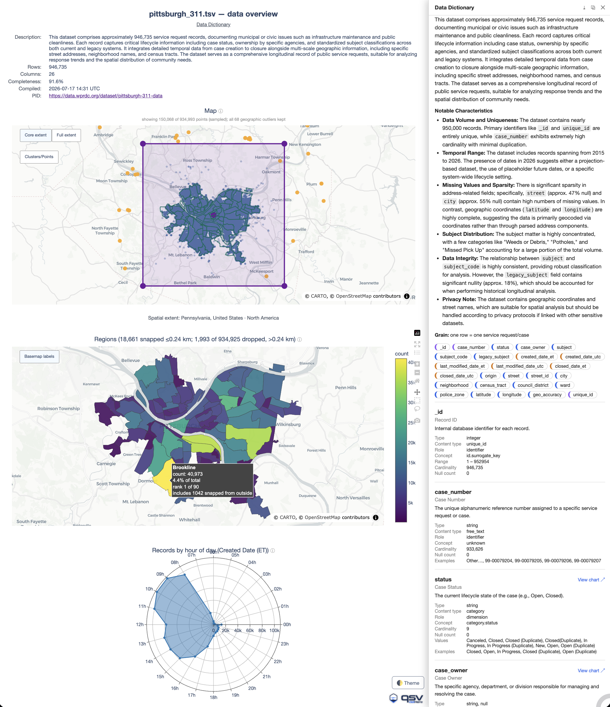
`qsv viz smart pitt311data.csv --smarter --dictionary pitt311data.schema.json \ --dict-info --bivariate -o pitt311data-smart-visual-datadic.html \ --geojson pittsburgh-neighborhoods --dataset-pid https://data.wprdc.org/dataset/pittsburgh-311-data`